Introduction

In this post, we shall deep dive into Tensorflow support for Differentiation using Gradient Tapes. Further explore the equations programmatically to understand the underlying capability.

In general differentiation can be accomplished through 4 techniques,

• Manual Differentiation
• Numerical Differentiation (ND)
• Symbolic Differentiation (SD)
• Automatic Differentiation (AutoDiff)

Both Numerical and Symbolic differentiations are considered as classical methods that are error prone. SD methods lead to inefficient code due to the challenges in converting a computer program into single expression. Meanwhile Numerical methods introduce round of errors due to discretization process(limits). Further, they are not suitable for gradient descent which is the backbone of Backpropation due to their inefficiency and performance bottleneck in computing partial derivatives.

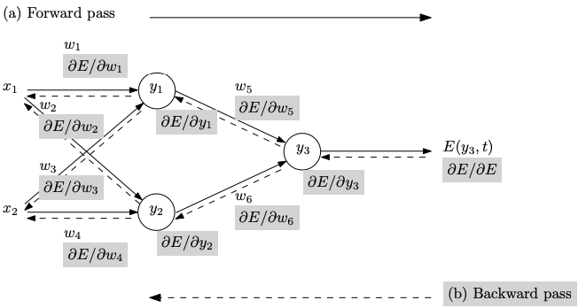
• Train inputs $x_i$ are fed forward, generating corresponding activations $y_i$
• An error E between the output $y_3$ and the target output $t$ is computed
• The error adjoint is propagated backward, giving the gradient with respect to the weights
  $\bigtriangledown_{wi}E = \left( \frac{\partial E}{\partial w_1}, \cdots, \frac {\partial E}{\partial w_6} \right)$
  which is subsequently used in a gradient-descent procedure
• The gradient wrt inputs $\bigtriangledown_{wi}E$ also be computed in the same backward pass

Image and Overview of Backpropagation Reference: Automatic Differentiation in Machine Learning: a Survey

Goal

I would consider the goal is accomplished, If one find answer to the following questions.

• What is Automatic Differentiation
• Where it is used?
• What is chain rule?
• How to find unknown differentiable equation from data?
• How to compute gradients?
• What is the significance of Gradient Tapes?
• Beyond equations, a programmatical implementation of the Auto Diff for few examples

Chain Rule

Chain rule is a formula to compute derivative of a composition of differentiable functions. To get an intuition, a differentiable function has a graph that is smooth and does not contain any break, angle or cusp. Chain rule is often confused due to its application both in Calculus and Probability(joint distribution, conditional probability and Bayesian networks).

$$\Large y = f(g(h(x)))) = f(g(h(w_{0}))) = f(g(w_{1})) = f(w_{2}) = w_{3}$$

Where, $w_0 = x$, $w_1 = h(w_0)$, $w_2 = g(w_1)$, $w_3 = f(w_2) = y$

then the chain rule gives
$\Large \frac{dy}{dx} = \frac{dy}{dw_2} \frac{dw_2}{dw_1} \frac{dw_1}{dx}$
$i.e$
$\Large \frac{dy}{dx} = \frac{df(w_2)}{dw_2} \frac{dg(w_1)}{dw_1} \frac{dh(w_0)}{dx}$

Accumulations Methods

There are two modes through which AutoDiff is performed,

1. Forward Accumuation and
2. Backward Accumuation - Used in Backpropagation of errors in Multi Layer Perceptron Deep Neural Networks

An equation worth millions compared to explanation of any kind in this quest.

Forward Accumulation

In forward accumulation, chain rule traverses from inside to outside
$\Large \frac{\partial y}{\partial x} = \frac{\partial y}{\partial w_{n-1}} \frac{\partial w_{n-1}}{dw_x}$

$\Large \frac{\partial y}{\partial x} = \frac{\partial y}{\partial w_{n-1}} \left(\frac{\partial w_{n-1}}{dw_{n-2}} \frac{\partial w_{n-2}}{dw_x} \right)$

$\Large \frac{\partial y}{\partial x} = \frac{\partial y}{\partial w_{n-1}} \left(\frac{\partial w_{n-1}}{dw_{n-2}} \left(\frac{\partial w_{n-2}}{dw_{n-3}} \frac{\partial w_{n-3}}{dw_x} \right) \right) = \dots$

Reverse Accumulation

In reverse accumulation, chain rule traverses from outside to inside

$\Large \frac{\partial y}{\partial x} = \frac{\partial y}{\partial w_1} \frac{\partial w_1}{dw_x}$

$\Large \frac{\partial y}{\partial x} = \left( \frac{\partial y}{\partial w_2} \frac{\partial w_2}{dw_1} \right) \frac{\partial w_1}{dw_x} $

$\Large \frac{\partial y}{\partial x} = \left( \left( \frac{\partial y}{\partial w_3}\frac{\partial w_3}{dw_2}\right) \frac{\partial w_2}{dw_1} \right) \frac{\partial w_1}{dw_x} = \dots$

Automatic Differentiation using Tensorflow

We saw what is a differential equation, we also pondered the salience of Backward accumulation in Multi Layer Perceptrons. Our goal for a Deep Neural Network(DNN) model is to minimize the error of an unknown differentiable equation. What is this unknown differentiable equation is a separate topic for an other day.

Minimizing the error is achieved by finding a local minima of the differentiable equation iteratively using an optimization algorithm. This process is called as Gradient Descent. For few other problems, we might change the direction and find the local maxima and that process is called as Gradient Ascent.

During DNN training, two operations occurs Forward Pass and Backward Pass. To differentiate automatically, one need to remember what happened during the forward pass and while traversing back these operations happened are reversed to compute gradients. Tensorflow provides Gradient tapes to remember, A right analogy is like our olden day VHS tapes. Things are recorded at every step of training and can be reversed just by traversing back.

Gradient Tapes

Tensorflow provided tf.GradientTape API for automatic differentiation to compute the gradient of certain inputs by recording the operations executed inside certain context. We shall examine this with few examples

Calculate Derivatives

Let us see, how to calculate derivative for this simple equation $$\frac{d}{dx}x^3 =3x^2$$ $$f’(x=1) = 3$$ $$f’(x=3) = 27$$

import numpy as np
import tensorflow as tf

def derivative(value):
    x = tf.Variable([[value]])
    with tf.GradientTape() as tape:
        loss = x * x * x
        
        dy_dx = tape.gradient(loss, x)

    return dy_dx

derive_1 = derivative(1.0)
derive_3 = derivative(3.0)

print(f'f\'(𝑥=1) = {derive_1.numpy()}')
print(f'f\'(𝑥=3) = {derive_3.numpy()}')

f'(𝑥=1) = [[3.]]
f'(𝑥=3) = [[27.]]

Calculate Derivative by Partial for Higher Rank Matrix

Let us say, We have a matrix of shape $2 \times 2$. That can be represented as $eqn.2$. We want to find the derivative of the square of that matrix. This is best done using partial derivative by assigning to a third variable $z$ ref $eqn.2$ $$y = \sum x$$ $$y=x_{1,1} + x_{1,2} + x_{2,1} + x_{2,2} \tag{1}$$ $$z=y^2\tag{2}$$

x = tf.ones((2, 2))
x

<tf.Tensor: shape=(2, 2), dtype=float32, numpy=
array([[1., 1.],
       [1., 1.]], dtype=float32)>

From the chain rule

$$\frac{\partial z}{\partial x} = \frac{\partial z}{\partial y} \times \frac{\partial y}{\partial x}$$ from equation 2 $$\frac{\partial z}{\partial y} = 2 \times y = 8$$ from equation 1 $$\frac{\partial y}{\partial x}= \frac{\partial y}{\partial x_{1,1}}, \frac{\partial y}{\partial x_{1,2}}, \frac{\partial y}{\partial x_{2,1}}, \frac{\partial y}{\partial x_{2,2}}$$ $$\frac{\partial y}{\partial x}= [[1, 1], [1, 1]] $$ hence $$\frac{\partial z}{\partial x} = \frac{\partial z}{\partial y} \times \frac{\partial y}{\partial x}$$ $$\frac{\partial z}{\partial x} = 8 \times [[1, 1], [1, 1]] = [[8, 8], [8, 8]]$$

with tf.GradientTape() as tape:
    tape.watch(x)
    y = tf.reduce_sum(x)
    z = tf.square(y)
    
dz_dx = tape.gradient(z, x)

dz_dx

<tf.Tensor: shape=(2, 2), dtype=float32, numpy=
array([[8., 8.],
       [8., 8.]], dtype=float32)>

Derivatives for Higher Degree Polynomial Equation

Let $x = 2$ and the 2nd degree polynomial equations as follows.

$$y = x^2 \tag{3}$$ $$z = y^2 \tag{4}$$

Using chain rule, Let us solve the derivative

$$\frac{\partial z}{\partial x} = \frac{\partial z}{\partial y} \times \frac{\partial y}{\partial x}$$ from equation 2 $$\frac{\partial z}{\partial y} = 2 \times y = 2 \times 3^2 = 18$$ $$\frac{\partial y}{\partial x} = 2x = 2 \times 3 = 6 \tag{5}$$ hence $$\frac{\partial z}{\partial x} = \frac{\partial z}{\partial y} \times \frac{\partial y}{\partial x} = 18 \times 6 = 108 \tag{6}$$

Solve the same by substitution $$\frac{\partial z}{\partial x}= \frac{\partial}{\partial x}x^4$$ $$\frac{\partial z}{\partial x}= 4x^3 = 4 \times 3^3 = 108 $$

x = tf.constant(3.0)
with tf.GradientTape(persistent=True) as tape:
    tape.watch(x)
    y = x ** 2
    z = y ** 2
    
dz_dx = tape.gradient(z, x)
dy_dx = tape.gradient(y, x)

print(f'∂𝑧/∂𝑥: {dz_dx}, ∂𝑦/∂𝑥: {dy_dx}')

∂𝑧/∂𝑥: 108.0, ∂𝑦/∂𝑥: 6.0

Derivative of Derivative

$$y=x^3$$ $$\frac{\partial y}{\partial x} = 3x^2$$ $$\frac{\partial^2 y}{\partial x^2}=6x$$

def derivative_of_derivative(x):
    x = tf.Variable(x, dtype=tf.float32)
    with tf.GradientTape() as tape_2:
        with tf.GradientTape() as tape_1:
            y = x ** 3
        dy_dx = tape_1.gradient(y, x)
    d2y_dx2 = tape_2.gradient(dy_dx, x)
    
    return dy_dx, d2y_dx2

dy_dx, d2y_dx2 = derivative_of_derivative(1)
print(f'x=1 -- ∂𝑦/∂𝑥: {dy_dx}, ∂2𝑦∂𝑥2: {d2y_dx2}')

dy_dx, d2y_dx2 = derivative_of_derivative(5)
print(f'x=5 -- ∂𝑦/∂𝑥: {dy_dx}, ∂2𝑦∂𝑥2: {d2y_dx2}')

x=1 -- ∂𝑦/∂𝑥: 3.0, ∂2𝑦∂𝑥2: 6.0
x=5 -- ∂𝑦/∂𝑥: 75.0, ∂2𝑦∂𝑥2: 30.0

Finding Unknown Differentiable Equation

Let us extract this function programmatically using tf.GradientTapes

$$y = 2x - 8 $$ $$\frac{dy}{dx} = 2 $$

Let us recreate this using numpy and tensorflow gradient tapes

x = np.array(np.random.choice(15, size=10, replace=False), dtype=float)
y = 2 * x - 8
print(f"x: {x}\ny: {y}")

x: [ 8. 10.  6.  3.  7.  9. 13.  1.  0. 11.]
y: [ 8. 12.  4. -2.  6. 10. 18. -6. -8. 14.]

We have the data pattern for the above said equation. Through this dataset, let us find the equation by performing following steps

• The above equation is of the form $y = mx + b$, each instance is a point on the 2D plane that connects and forms a line $$y = mx + b$$
• We have to train the variable $m$ the coefficient and $b$ the intercept. $m$ and $b$ using tf.Variable
• As mentioned above, our goal is the minimize the error by using an optimization function. A loss($loss_{fn}$) function using tf.abs of predicted $\hat y$ and actual $y$
• We have to compute this through multiple iterations. A fit functions using tf.GradientTape by iterating for EPOCHS time
• We also have a LEARNING RATE that is a constant

LEARNING_RATE = 0.001
m = tf.Variable(np.random.random(), trainable=True)
c = tf.Variable(np.random.random(), trainable=True)

def loss_fn(y, y_hat):
    return tf.abs(y - y_hat)

def fit(x, y):
    with tf.GradientTape(persistent=True) as tape:
        # Predict y from data
        y_hat = m * x + c
        
        # Calculate the loss
        loss = loss_fn(y, y_hat)
        
    # Calculate Gradients
    m_gradient = tape.gradient(loss, m)
    c_gradient = tape.gradient(loss, c)
    
    # Update the Gradient and apply learning 
    m.assign_sub(m_gradient * LEARNING_RATE)
    c.assign_sub(c_gradient * LEARNING_RATE)

EPOCHS = 2000
for i in range(EPOCHS):
    fit(x, y)
    if(i % 100 == 0):
        print(f'EPOCH: {i:04d}, m: {m.numpy()}, c: {c.numpy()}')

EPOCH: 0000, m: 0.6082303524017334, c: 0.19983896613121033
EPOCH: 0100, m: 1.1402301788330078, c: -0.1361609399318695
EPOCH: 0200, m: 1.1762301921844482, c: -0.532161295413971
EPOCH: 0300, m: 1.2302302122116089, c: -0.9261620044708252
EPOCH: 0400, m: 1.2662302255630493, c: -1.3221579790115356
EPOCH: 0500, m: 1.3022302389144897, c: -1.7181528806686401
EPOCH: 0600, m: 1.3562302589416504, c: -2.1121480464935303
EPOCH: 0700, m: 1.3922302722930908, c: -2.508143186569214
EPOCH: 0800, m: 1.4462302923202515, c: -2.9021384716033936
EPOCH: 0900, m: 1.482230305671692, c: -3.298133611679077
EPOCH: 1000, m: 1.5362303256988525, c: -3.692128896713257
EPOCH: 1100, m: 1.572230339050293, c: -4.08812952041626
EPOCH: 1200, m: 1.6262303590774536, c: -4.482147216796875
EPOCH: 1300, m: 1.662230372428894, c: -4.878165245056152
EPOCH: 1400, m: 1.6982303857803345, c: -5.27418327331543
EPOCH: 1500, m: 1.7522304058074951, c: -5.668200969696045
EPOCH: 1600, m: 1.7882304191589355, c: -6.064218997955322
EPOCH: 1700, m: 1.8402304649353027, c: -6.458236217498779
EPOCH: 1800, m: 1.884230613708496, c: -6.8522515296936035
EPOCH: 1900, m: 1.9182307720184326, c: -7.246265888214111

print(f"y ~ {m.numpy()}x + {c.numpy()}")

y ~ 1.9022306203842163x + -7.554266452789307

Hence, $$\Huge y \sim 1.92x - 7.22$$ $$\Huge \simeq$$ $$\Huge y = 2x - 8 $$

Inference

1. Have we found the polynomial function programmatically using Gradient Tapes? - YES
2. Are we able to differentiate polynomial equation of various degrees? - YES
3. Are we able to compute gradeints using Gradient Tape? - Yes
4. Have we established the relationship between Chain Rule and Gradient Descent? - YES
5. Have we achieved our goals? - If YES, I request you to promote this blog by a tweet or a linkedin share. It means a lot to me.

Thank You

References

Automatic Differentiation and Gradients
Differentiable Functions
Automatic Differentiation in Machine Learning: a Survey