We are revisiting Gradient Descent for optimizing a Gaussian Distribution using Jacobian Matrix. This post covers partial derivatives, differential equations, optimizations and a good number of visualizations on optimization and convergence. Following are the related posts,

• Automatic Differentiation Using Gradient Tapes
• Roll your sleeves! Let us do some partial derivatives.

Image Credit: https://besthqwallpapers.com/

Objective

We try to get a clarity on the following questions

• What is gradient?
• How gradient descent/ascent achieved
• What are critical points and how they impact convergence?
• Global, local maximas and minimas and saddle points
• Multivariate functions and gradient calculation for them
• What is a Jacobian matrix, significance of Jacobians in optimization
• Gradient descent for Regression using Ordinary Least Square method
• Non-linear regression optimization using Jacobian matrix
• Simulation of Gaussian Distribution and convergence scheme

Introduction

Gradient is the slope of a differentiable function at any given point, it is the steepest point that causes the most rapid descent. As discussed above, minimizing the error is our goal and we have to achieve that goal through the cost function which is a differentiable one.

On a 2D plane for a differentiable function $f(x)$, gradient at a point $x$ is

$$\text{Gradient at }x = f’(x) = \frac {df}{dx} = \frac {f(x + \Delta x) - f(x)} {(x + \Delta x) - x}$$ $$i.e.$$ $$f’(x) = = \frac {f(x + \Delta x) - f(x)} {\Delta x}$$ when $\Delta x$ tend to go almost to zero, $$f’(x) = \lim_{\Delta x \rightarrow 0} \left (\frac {f(x + \Delta x) - f(x)} {\Delta x} \right) \tag{1. Gradient}$$

i.e Our cost function is the destination for our journey and the gradient provides the direction of the journey. Direction of our journey is determined by the sign of the derivative

$$sign(x)=\begin{cases} -1 & if x < 0, descent \ 0 & if x = 0 \ 1 & if x > 0, ascent \end{cases} \tag{2. Direction}$$ then this journey is $$f(x + \Delta x) \approx f(x) + \Delta x f’(x) \tag{3. Gradient Ascent}$$ $$f(x - \Delta x) \approx f(x) - \Delta x f’(x) \tag{4. Gradient Descent}$$

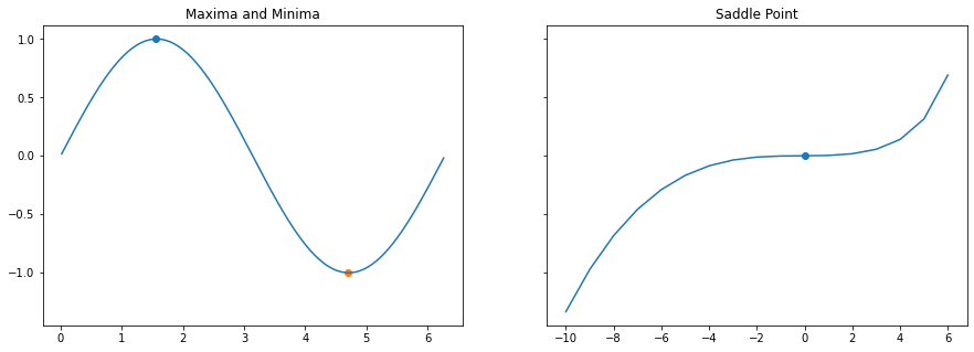
Critical Points: Minima, Maxima and Saddle Point

Critical points are the ones where our destination lies, ie It’s like climbing or descenting a hill.. while making this journey we come across 3 interesting locations

1. Maximas - Peaks of the journey
2. Minimas - Deepest location of the journey
3. Saddle Points - Plateaus where we get confused about the direction

Trivia.

• Gradient of a horizontal line is zero($0$)
• Gradient of a straight line is same at all points
• A climb(ascent) has positive gradient and a fall(descent) has negative slope.

Finding these points accurately makes a machine learning algorithm an accurate one.

import numpy as np
import matplotlib.pyplot as plt

fig, axs = plt.subplots(1, 2, figsize=(15, 5), sharey=True)
x = np.arange(1, 360, 1) * np.pi / 180.
y = np.sin(x)
axs[0].plot(x, y)
axs[0].scatter(1.55, 1)
axs[0].scatter(4.7, -1)
axs[0].set_title("Maxima and Minima")

x1 = np.arange(-10, 7, 1)
y1 = (4 * x1**3 - np.cos(x1) + 3 * np.exp(x1)) / 3000
axs[1].plot(x1, y1)
axs[1].scatter(0, 0)
axs[1].set_title("Saddle Point")

plt.show()

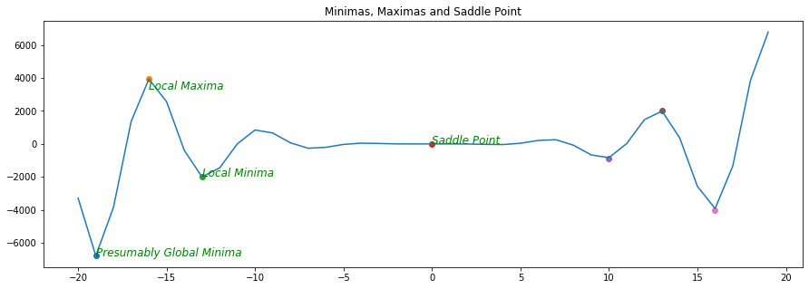
Multiple Minimas

When there are more than one minimas or saddle points - often the optimization alogrithms fails. Escaping from a saddle point is a deep topic of research and this article just introduces what exactly they are.

x1 = np.arange(-20, 20, 1)
y = np.arange(-20, 20, 1)
plt.figure(figsize=(15, 5))
y1 = x1**3 * np.cos(x1) - x1 * np.sin(x1)
plt.plot(x1, y1)
points = [[-19, -6784], [-16, 3927.19], [-13, -2000], [0, 0], [10, -900], [13, 2000], [16, -4000]]
[plt.scatter(pt[0], pt[1]) for pt in points]

plt.text(-19, -6784, 'Presumably Global Minima', style ='italic',
        fontsize = 12, color ="green")
plt.text(-13, -2000, 'Local Minima', style ='italic',
        fontsize = 12, color ="green")
plt.text(-16, 3296, 'Local Maxima', style ='italic',
        fontsize = 12, color ="green")
plt.text(0, 0, 'Saddle Point', style ='italic',
        fontsize = 12, color ="green")
plt.title("Minimas, Maximas and Saddle Point")
plt.show()

Multivariate Functions

Until now we saw univariate functions where the outcome is decided by a single variable. However machine learning systems are multi-dimensional and we often come across complex cost function functions. Let us say, we have a function with multiple variables $f(x_1, x_2, x_3, \cdots, x_n)$ i.e. the features of the dataset then the derivative of that function becomes quite difficult. This is addressed through partial derivatives as follows…

Let us say we have 3 variables $x, y, z$ in our dataset then our differentiable function is $$f(x, y, z)$$ $$then$$ $$f’(x, y, z) = \frac{\partial f }{\partial x} + \frac{\partial f }{\partial y} + \frac{\partial f }{\partial z}$$ i.e. We can differentiate anything with respect to anything. We represent these partial derivatives in matrix form and it is called as Jacobian Matrix. $$J = \left [ \frac{\partial f }{\partial x}, \frac{\partial f }{\partial y}, \frac{\partial f }{\partial z} \right]$$ Jacobian is a row vector. We can generalize this as follows $$f(x_1, x_2, x_3, \cdots, x_n)$$ $$then$$ $$J(x_1, \cdots, x_n) = \nabla_x f(x) = \left [ \frac{\partial f }{\partial x_1}, \frac{\partial f }{\partial x_2}, \frac{\partial f }{\partial x_3}, \cdots, \frac{\partial f }{\partial x_n} \right] \tag{5. Jacobian Matrix}$$ Further, Jacobian is a vector that we can calculate for each and every location on the space. The steeper the slope, the greater the magnitude of the Jacobian.

Critical points are the locations where every element of the gradient is equal to zero,

$$\nabla_x f(x) = 0 = \begin{cases} \frac{\partial f}{\partial x_1} = 0 \ \frac{\partial f}{\partial x_2} = 0 \ \vdots \ \frac{\partial f}{\partial x_n} = 0 \end{cases} \tag{6. Critical Point}$$

Gradient Descent for Regression

In this section, we shall explore regression problem using Ordinary Least Square methods. OLS are the best methods for residual analysis, where it penalises when the errors are large. This section has an overview to linear regression and in depth implementation of non-linear regression for a Gaussian Distribution.

Linear Least Squares

We shall start our Linear Regression from the equation of a line $y=mx+c$ as follows

$$y = y(x;a_i) = mx_i + c$$ then the residual of the fitted line is $r_i$ and the overall efficacy of the fitted line is $\chi^2$. i.e. $$\chi^2 = \sum_{i=0}^n r_i^2 = \sum_{i=0}^n (y_i - mx_i - c)^2 \tag{7. Chi-Squared loss}$$ where there are $n$ observersions.

Jacobian of Chi-Squared Loss

Our goal is to identify the right value for the gradient(slope) $m$ and the intercept $c$. Let us do partial derivative of the loss function wrt $m, c$ to make a Jacobian matrix.

from $equ.7$, differentiate wrt $m$ $$\frac{\partial \chi^2}{\partial m} = \sum_i 2 * (y_i - mx_i - c)^{2-1} * -x_i$$ $$i.e$$ $$\frac{\partial \chi^2}{\partial m} = -2\sum_i x_i(y_i - mx_i - c)$$

from $equ.7$, differentiate wrt $c$ $$\frac{\partial \chi^2}{\partial c} = \sum_i 2 * (y_i - mx_i - c)^{2-1} * -1$$ $$i.e$$ $$\frac{\partial \chi^2}{\partial c} = -2\sum_i (y_i - mx_i - c)$$

$$hence \ the \ jacobian \ matrix \ is$$ $$\nabla \chi^2 = \left( \begin{array}{cc} \frac{\partial{\chi^2}}{\partial{m}}, \ \frac{\partial \chi^2}{\partial c} \end{array} \right) = \left( \begin{array}{cc} -2\sum_i x_i(y_i - mx_i - c), \ -2\sum_i (y_i - mx_i - c) \end{array} \right) \tag{8. Jacobian for Linear Regression}$$

Refer, a complete implementation of Linear Lease Squares is demonstrated using Tensorflow Gradient Tapes in this post

• Finding Unknown Differentiable Equation

Non Linear Least Squares

We shall examine a non linear function of Gaussian distribution with 4 fitting parameters $(\sigma, \mu, I, b)$ and build a Jacobian matrix. $$\Large y(x; \sigma, \mu, I, b) = b + \frac {I}{\sigma\sqrt{2\pi}} e^{ \left( - \frac{(x - \mu)^2}{2\sigma^2} \right) }$$

def gaussian(x, mu, sigma, I=1, b=0):
    return b + I * np.exp(-(x-mu)**2/(2*sigma**2)) / (np.sqrt(2*np.pi) * sigma)

Jacobian of Gaussian Function

then it’s Jacobian Matrix is $$\Large \nabla \chi^2 = \left[\begin{array}{cc} \frac{\partial \chi^2}{\partial \sigma} \ \frac{\partial \chi^2}{\partial \mu} \ \frac{\partial \chi^2}{\partial I} \ \frac{\partial \chi^2}{\partial b} \end{array}\right] $$

The following derivative is done by hand,

$$\frac{\partial \chi^2}{\partial \sigma} = \frac {I}{\sigma\sqrt{2\pi}} e^{ \left( - \frac{(x - \mu)^2}{2\sigma^2} \right) } * \left(\frac{(x-\mu)^2}{\sigma^3} - \frac{1}{\sigma} \right)$$

$$\frac{\partial \chi^2}{\partial \mu} = \frac{I}{\sqrt{2\pi}} \frac{(x - \mu)}{\sigma^3} e^{ \left( - \frac{(x - \mu)^2}{2\sigma^2} \right) }$$

$$\frac{\partial \chi^2}{\partial I} = \frac {1}{\sigma\sqrt{2\pi}} e^{ \left( - \frac{(x - \mu)^2}{2\sigma^2} \right) }$$

$$\frac{\partial \chi^2}{\partial b} = 1$$

and the Jacobian matrix for the Gaussian Distribution as follows

$$\nabla \chi^2 = \left[\begin{array}{cc} \frac{\partial \chi^2}{\partial \sigma} \ \frac{\partial \chi^2}{\partial \mu} \ \frac{\partial \chi^2}{\partial I} \ \frac{\partial \chi^2}{\partial b} \end{array}\right] = \left[\begin{array}{cc} \frac {I}{\sigma\sqrt{2\pi}} e^{ \left( - \frac{(x - \mu)^2}{2\sigma^2} \right) } * \left(\frac{(x-\mu)^2}{\sigma^3} - \frac{1}{\sigma} \right), \ \frac{I}{\sqrt{2\pi}} \frac{(x - \mu)}{\sigma^3} e^{ \left( - \frac{(x - \mu)^2}{2\sigma^2} \right) }, \ \frac {1}{\sigma\sqrt{2\pi}} e^{ \left( - \frac{(x - \mu)^2}{2\sigma^2} \right) }, \ 1 \end{array}\right] \tag{9. Jacobian of Gaussian Distribution}$$

Build the Partial Derivatives

There are four fitting parameters $(\sigma, \mu, I, b)$, We shall build four methods that accomplish partial derivatives wrt them

• $\frac{\partial \chi^2}{\partial \sigma}$ - dchi2_dsigma
• $\frac{\partial \chi^2}{\partial \mu}$ - dchi2_dmu
• $\frac{\partial \chi^2}{\partial I}$ - dchi2_dI
• $\frac{\partial \chi^2}{\partial b}$ - dchi2_db

# ∂𝜒2/∂𝜎
def dchi2_dsigma(x, mu, sigma, I=1, b=0):
    return gaussian(x, mu, sigma, I, b) * (((x-mu)**2 / sigma**3) - (1/sigma))

# ∂𝜒2/∂𝜇
def dchi2_dmu(x, mu, sigma, I=1, b=0):
    return gaussian(x, mu, sigma, I, b) * ((x-mu) / sigma**2)

# ∂𝜒2/∂𝐼
def dchi2_dI(x, mu, sigma, I=1, b=0):
    return np.exp(-(x-mu)**2/(2*sigma**2)) / (np.sqrt(2*np.pi) * sigma)

# ∂𝜒2/∂𝑏
def dchi2_db(x, mu, sigma, I=1, b=0):
    return 1

Ordinary Differential Equation - Step Function

Single step of length $(\sigma, \mu, I, b)$ is multiplied to solve the differential equation.

def step_fn(x, y, mu, sig, I=1, b=0, aggression=2000):
    J = np.array([
        -2 * (y - gaussian(x, mu, sig)) @ dchi2_dmu(x, mu, sigma),
        -2 * (y - gaussian(x, mu, sig)) @ dchi2_dsigma(x, mu, sigma),
        -2 * (y - gaussian(x, mu, sig)) @ dchi2_dI(x, mu, sigma),
        -2 * (y - gaussian(x, mu, sig)) * dchi2_db(x, mu, sigma)
    ])

    step = -J * aggression
    return step

def ode(x, y_init, mu_pred, sigma_pred, I_pred, b_pred):
    preds = np.array([[mu_pred, sigma_pred, I_pred, b_pred]])
    for i in range(100):
        dmu, dsigma, dI, db = step_fn(x, y_init, mu_pred, sigma_pred, I_pred, b_pred, 2000)
        mu_pred += dmu
        sigma_pred += dsigma
        I_pred += dI
        b_pred += db
        preds = np.append(preds, [[mu_pred, sigma_pred, I_pred, b_pred]], axis=0)

    return preds, mu_pred, sigma_pred, I_pred, b_pred

Simulations

Let us build helper functions to create and visualize the distributions and convergence.

def plot_distributions(x, y, y_init):
    fig, axs = plt.subplots(1, 2, figsize=(20, 5), sharey=True)
    axs[0].plot(x, y)
    axs[0].set_title("Actual Distribution")
    axs[1].plot(x, y_init, color="green")
    axs[1].set_title("Initial Distribution for Prediction")

    plt.show()

def create_distribution(x, mu_init = 25, sigma_init = 3):
    mu = np.mean(x)
    sigma = np.std(x)
    y = gaussian(x, mu, sigma)
    y_init = gaussian(x, mu_init, sigma_init)

    return x, y, mu, sigma, y_init, mu_init, sigma_init

def compare_distributions(x, y, y_pred):
    plt.figure(figsize=(10, 5))
    plt.ylim([0, 0.02])
    plt.plot(x, y, label="Actual Distribution")
    plt.plot(x, y_pred, label="Predicted Distribution")
    plt.legend()
    plt.show()

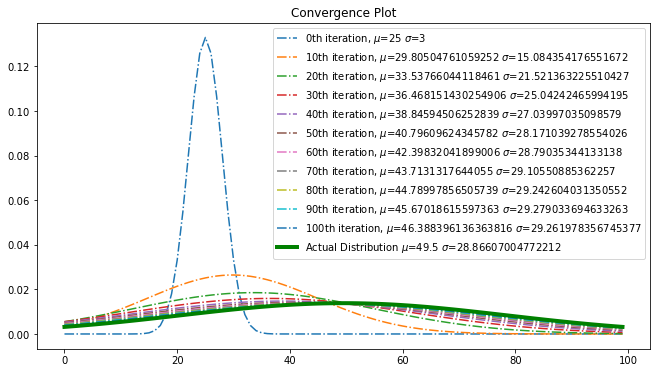
def convergence_plot(x, y, preds):
    plt.figure(figsize=(11, 6))

    for i in np.arange(0, len(preds)):
        if(i % 10 == 0):
            y1 = gaussian(x, preds[i][0], preds[i][1])
            plt.plot(x, y1, label=f"{i}th iteration, $\mu$={preds[i][0]} $\sigma$={preds[i][1]}", linestyle='dashdot')
            plt.legend()
    plt.plot(x, y, color="green", linewidth=4, label=f"Actual Distribution $\mu$={mu} $\sigma$={sigma}")
    plt.legend()
    plt.title("Convergence Plot")
    plt.show()

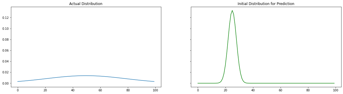
Actual and Initial Distributions

We are creating two distribution, 1 is the actual data and the other one initialized with a random mean($\mu_{actual}$) and random standard deviation($\sigma_{actual}$). Our goal is to used the data of the first distribution and predicted ($\mu_{pred}, \sigma_{pred}$). Let us compare the actual and initial distributions visually.

x, y, mu, sigma, y_init, mu_init, sigma_init = create_distribution(np.arange(0, 100, 1))
plot_distributions(x , y, y_init)

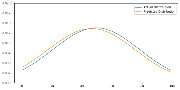
Predicted Disribution

Using our ODE iterator function, we have calculated ($\mu_{pred}, \sigma_{pred}$). Using new mean and standard deviation, $y_{pred}$ calculated and visualization aligns with very minimal error.

I_init = 1
b_init = 0
preds, mu_pred, sigma_pred, I_pred, b_pred = ode(x, y, mu_init, sigma_init, I_init, b_init)
y_pred = gaussian(x, mu_pred, sigma_pred)
compare_distributions(x, y, y_pred)

<ipython-input-5-af1d68394805>:2: VisibleDeprecationWarning: Creating an ndarray from ragged nested sequences (which is a list-or-tuple of lists-or-tuples-or ndarrays with different lengths or shapes) is deprecated. If you meant to do this, you must specify 'dtype=object' when creating the ndarray
  J = np.array([
<__array_function__ internals>:5: VisibleDeprecationWarning: Creating an ndarray from ragged nested sequences (which is a list-or-tuple of lists-or-tuples-or ndarrays with different lengths or shapes) is deprecated. If you meant to do this, you must specify 'dtype=object' when creating the ndarray

Convergence

Using convergence plot, examine the step wise convergence to reach the optimal point.

convergence_plot(x, y, preds)

Inference

The most significant aspect of this post is not using any sophisticated packages to calculate the gradient descent. This is more a proof of the efficacy of Jacobian matrix in optimization challenges. This post is an incomplete one, I planned to add the following topics in the futre posts

• Hessian Matrix for learning rate determination and measure of curvature
• Eigen values, vectors and spaces: One of my favorite topics
• Taylors series, Newton Raphson method and Lagrange Multipliers

References

• What is the difference between the Jacobian, Hessian and the gradient in machine learning? by Ivan Davis, 2019
• Gradient Descent from Wikipedia
• Jacobian matrix and determinant