We shall see, how KL-Divergence works for Cats and Dogs classification problem.

Image Credit: www.mentalfloss.com

Previous Posts in this Series

• Bayesian and Frequentist Approach to Machine Learning Models
• Understaning Uncertainty, Deterministic to Probabilistic Neural Networks
• Shannon’s Entropy, Measure of Uncertainty When Elections are Around

Objective

Our objective is to get answers to the following questions

• What is KL Divergence?
• Why log likelihood?
• What is Likelihood ratio?
• Is expected values - Weighted average of instances of Random values?
• Is expected value of log likelihood ratio is KLD?
• What can KL-Divergence be used for?
• How are KL-Divergence and Cross Entropy related?
• Is KL-Divergence a distance measure?
• How are KL-Divergence and Log-Likelihood related?
• Is KLD asymmetric?
• What are forward and reverse KL?

Introduction

KL-Divergence is a measure of how two distributions differ from each others. Some of very well known probability density distribution plots

Image Credit: ∫ntegrabℓε ∂ifferentiαℓs

Let us say we are building a deep neural network that classifies dogs and cats, for a dog picture - The probability of classifying a dog as dog by a perfect neural network is 1. i.e

$$\large p_{\theta}(dog) = 1, p_{\theta}(cat) = 0$$ where $\theta$ represents the reality.

Network Performance
However, our neural networks is governed by the estimated weights $\phi$. i.e for a decent neural network, outcome could be $$\large q_{\phi}(dog) = 0.8, q_{\phi}(cat) = 0.2$$ Meanwhile, if our network behaves adversarial to the expectations… we seek deeper explanations. i.e. $$\large q_{\phi}(dog) = 0.2, q_{\phi}(cat) = 0.8$$

Hence, we seek a clarity to declutter this uncertainity by measuring the probabilities relatively.

KL-Divergence

In the above representations, we introduced two probabilities $p_{\theta}$ representing the distribution of the reality and $q_{\phi}$ representing the distribution of the estimator(DNN).

From a dataset $X$ with observations ${x_1, x_2, x_3, \cdots, x_n}$, the probability for a single observation($i$) can be written as below as a representation of two distributions, $$p_{\theta}(x_i), q_{\phi}(x_i)$$

A typical measure of difference is subtracting $p_{\theta}$ and $q_{\phi}$ but we are dealing with very small numbers which might result in rounding to zero. To avoid this, we compute log differences or loglikelihood. i.e instead of $$p_{\theta}(x_i) - q_{\phi}(x_i)$$ We take logarithmic difference $$log p_{\theta}(x_i) - log q_{\phi}(x_i)$$ $$i.e.$$ $$\large log \frac { p_{\theta}(x_i)}{q_{\phi}(x_i)} \tag{1. Log Likelihood Ratio}$$

We saw the behavior for a single observer $i$ but our interest is to understand the likelihood of the whole sample set. Which is what is the average likelihood or the tendency of the random variables

KLD from Expected Value for Discrete Random Variables

Since every observation has a role in determining the probability, we have to give give importance to the ones with maximum likelihood. Hence a weighted average to all the observations are computed

$$\mathbb{E_{p\theta}}[h(X)] = \sum_{i=1}^\infty h(x_i)p_{\theta}(x_i) \tag{2. Expected Values}$$

Our goal is to find the average difference between the distributions $p_{\theta}$ and $q_{\phi}$, here expected values comes handy to calculate the average log likelihood ratio.

from eq.1 and eq.2

$$\sum_{i=1}^{\infty}p_{\theta}(x_i)log \frac {p_{\theta}(x_i)}{q_{\phi}(x_i)} \tag{3. Expected Log Likelihood Ratio}$$ $$i.e.$$ $$\large \mathbb{E_p}\left[log \frac {p_{\theta}(x)}{q_{\phi}(x)}\right ] = \sum_{i=1}^{\infty}p_{\theta}(x_i)\left[log \frac {p_{\theta}(x_i)}{q_{\phi}(x_i)}\right ] \tag{4. KL-Divergence}$$

Continuous Random Varaibles

For continuous random variables $$D_{KL}(p_{\theta} || q_{\phi}) = \int_{\mathbb{R}} p_{\theta}(x)\left[log \frac {p_{\theta}(x)}{q_{\phi}(x)}\right ]dx \tag{5. Forward KLD}$$ $$and$$ $$D_{KL}(q_{\phi} || p_{\theta}) = \int_{\mathbb{R}} q_{\phi}(x)\left[log \frac {q_{\phi}(x)}{p_{\theta}(x)}\right ]dx \tag{6. Reverse KLD}$$

They are not symmetric, i.e. $$D_{KL}(p_{\theta} || q_{\phi}) \neq D_{KL}(q_{\phi} || p_{\theta})$$ Hence it is not distance measure but divergence.

Generally $p$ is the reference distribution and $q$ is approximation. Forward KLs are the cross-entropy losses widely used in machine learning.

KL-Divergence as Loss Function

In this section let us explore how KL-Divergence is used as a loss function, from eqn.4

$$\large \sum_{i=1}^{\infty}p_{\theta}(x)log p_{\theta}(x) - \sum_{i=1}^{\infty}p_{\theta}(x)log q_{\phi}(x)$$

• The negative part is the cross-entropy $H(p_{\theta}, p_{\phi})$
• The positive part is the negative of entropy $H(p_{\theta}, p_{\theta})$, constant and derived from the dataset

Hence the loss function is $$\large - \sum_{i=1}^{\infty}p_{\theta}(x)log q_{\phi}(x)$$

Cats and Dogs

We created 2 situations out of our neural network,

1. With a decent outcome and $$q_{\phi}(dog) = 0.8, q_{\phi}(cat) = 0.2$$
2. With adversarial outcome $$q_{\phi}(dog) = 0.2, q_{\phi}(cat) = 0.8$$

Let us calculate KL-Divergence between reality and estimation

Image Credit: www.searchenginejournal.com

Case 1: $q_{\phi}(dog) = 0.8, q_{\phi}(cat) = 0.2$

$$1.log_2 \left[\frac {1.0}{0.8}\right] + 0.log_2 \left[\frac {1}{0.2} \right]$$ $$i.e.$$ $$0.3219$$

Observation: KLD value is closer to zero

Case 2: $q_{\phi}(dog) = 0.2, q_{\phi}(cat) = 0.8$

$$1.log_2 \left[\frac {1.0}{0.2}\right] + 0.log_2 \left[\frac {1}{0.8} \right]$$ $$i.e.$$ $$2.3219$$

Observation: KLD value is far from zero

Case 3: A perfect model

$$1.log_2 \left[\frac {1.0}{1.0}\right] + 0.log_2 \left[\frac {1}{0.0} \right]$$ $$i.e.$$ $$0$$

Observation: KLD value is zero since it is a perfect model

$$\sum_{i=1}^{\infty}p_{\theta}(x_i)log \frac {p_{\theta}(x_i)}{q_{\phi}(x_i)} \geq 0$$

When two disributions are similar then the KL-Divergence value is close to zero and it increases as the intensity of differences of distributions increases

import tensorflow as tf
import tensorflow_probability as tfp
tfd = tfp.distributions
tfb = tfp.bijectors

import matplotlib.pyplot as plt

Computing KL Divergence

In this section we shall explore how to use KL-Divergence API from Tensorflow Probabilities module

Univariate Gausian Distributions

Let us compute KL divergence for two univariate normal distributions using Tensorflow Probabilities functions.

• Create $p$ and $q$ distributions, using $\mu = { 1, 2 }$ and $\sigma={ 1, 0.5 }$
• Compute the divergence using tensorflow distributions

𝜇_q = 1
𝜎_q = 1
𝜇_p = 2
𝜎_p = 0.5

distribution_q = tfd.Normal(loc=𝜇_q, scale=𝜎_q)
distribution_p = tfd.Normal(loc=𝜇_p, scale=𝜎_p)

n_samples = 1000
samples_q = distribution_q.sample(n_samples)
samples_p = distribution_p.sample(n_samples)

plt.figure(figsize=(20, 5))
plt.subplot(1, 2, 1)
plt.hist(samples_q, bins=50, density=True)
plt.subplot(1, 2, 2)
plt.hist(samples_p, bins=50, density=True)
plt.show()

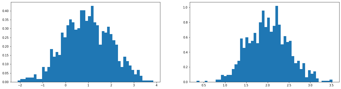
Observe the distribution mean and the spread in the above histograms. Further let us calculate the KL divergence

tfd.kl_divergence(distribution_q, distribution_p)

<tf.Tensor: shape=(), dtype=float32, numpy=2.8068528>

Asymmetry

Note when we swap the distribution KLD value varies, hence it is not a measure of distance but divergence

tfd.kl_divergence(distribution_p, distribution_q)

<tf.Tensor: shape=(), dtype=float32, numpy=0.6371457>

Fair Coin vs Unfair Coin

distribution_q = tfd.Categorical(probs=[0.5, 0.5])

distribution_p = tfd.Categorical(probs=[0.99, 0.01])

samples_q = distribution_q.sample(n_samples)
samples_p = distribution_p.sample(n_samples)

plt.figure(figsize=(20, 5))
plt.subplot(1, 2, 1)
plt.hist(samples_q, bins=3, density=True)
plt.subplot(1, 2, 2)
plt.hist(samples_p, bins=3, density=True)
plt.show()

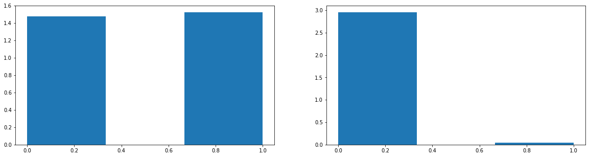
tfd.kl_divergence(distribution_q, distribution_p)

<tf.Tensor: shape=(), dtype=float32, numpy=1.6144631>

2 Fair Coins

tfd.kl_divergence(distribution_q, distribution_q)

<tf.Tensor: shape=(), dtype=float32, numpy=0.0>

Conclusion

In this post, we dived deep into KL-Divergence formula and how it is derived. Also learnt the significance of KL divergence in cross-entropy calculation. Further, we calculated KLD for various probability distributions understood the efficacy of the algorithm.

Reference

• tfp.distributions.kl_divergence
• Kullback–Leibler divergence
• What is KL Divergence?