Since nature is a non linear, reflexive, chaotic system and anticipating certainty will be limitting one’s potential in its forms or functions. Hence a deeper study of uncertainty is quite relevant in the context of machine learning and artificial intelligence.

In conventional deep learning models, the weigths are point functions of very minimal knowledge on the supporting dataset - This result in poor model performance, they are neither precise nor accurate. When the nature of all the problems are stochastic, a point function based inferential systems often result in uncertainties in the outcomes. This cause a compelling need to understand uncertainties in general and formalizing a boundary by disinguishing them to avoid more uncertainties.

This post is my class notes taken while attending Probabilistic Deeplearning Model course offered by Imperial College, London(Dr. Kevin Webster and team)

Image Credit: Dilbert

Objective

Following are the objectives of this post

1. Explore types of uncertainties and simulate them
2. Build deterministic and probabilistic models and compare their outcomes
3. Improve the probabilistive model to understand the distribution of uncertainties
4. Visualize the predicted probability distributions vs point function of deterministic model

Introduction

Awareness and understanding is the foundation for avoiding uncertainties. In this post

1. Create synthetic linear and non linear data to understand types of uncertainties
2. Build 3 different probabilistic models using Bayesian principles for regression to examine the outcomes
3. Compare the results with deterministic models

import utils as U
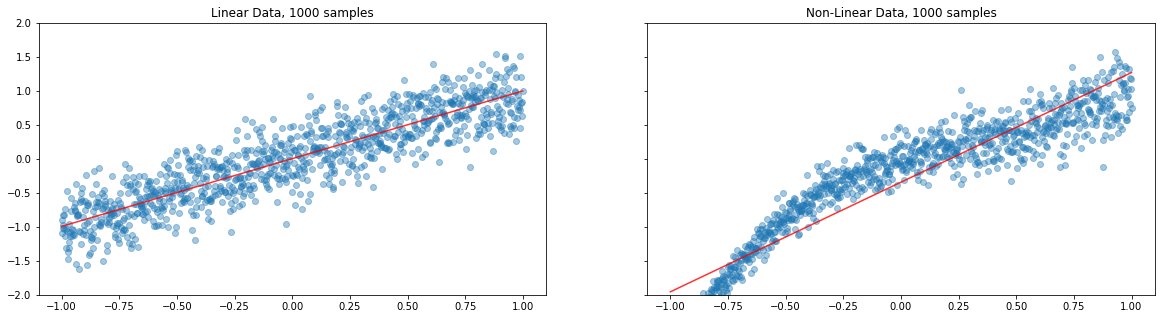
n_samples=1000
x_lin, y_lin, x_non_lin, y_non_lin = U.create_synthetic(n_samples)

We have created two sets of data and plotted above, each set has a feature vector and their respective target variables ie $(x, y)$. The first plot looks quite predictable and linear but the second one looks neither predictable nor linear. ie the dichotomy between the first and second plot is a function of uncertainty(or certainty) measure.

Nature of the above created data is

1. Linear data with Gaussian Noise
2. A Non-Linear data with a learned mean and variance

Classification of Uncertainties

Aleatoric Uncertainty

Aleatoric uncertainties are inherent part of the data itself, few examples

• Errors caused while measuring the data
• Noises in the environment that influence the data
• Randomness caused due to the nature data collection process These problems cannot avoided, they are always going to be there regardless of the model architecture.

There are two types of Aleatoric Uncertainty

• Homoscedastic: If the data uncertainty is same for all target variables regardless of the input, then it is homoscedastic
• Heteroscedastic: If the data uncertainty varies for the target variables according to the input, then it is heteroscedastic

Image Credit: Stack Exchange

Epistemic Uncertainty

Epistemic uncertainty is a function of feature parameters and data volume. ie as the number of observations and parameters grow, the measure of uncertainty naturally decreases. Due to this model explainability is quite possible by enhancing the ability to identify statistically significant parameters.

Image Credit: xkcd

In this post, we shall explore methods for identifying Aleatoric and Epistemic uncertainties using probablistic layers from TF probability.

Aleatoric Uncertainty

Let us create 3 tensorflow sequential models to demonstrate deterministic and probabilistic approach to deep neural networks and Aleatoric uncertainty.

• Determinisitc Linear Regression, A single layer sequential model with Mean Squared Error loss
• Probabilistic Linear Regression, A 2 layer sequential model with a normal distribution as final layer using Distribution Lambda function
• Probabilistic LR with Fixed Variance, A 3 layer sequential model with non linear learned mean and variance in the final layer.

import tensorflow as tf
import tensorflow_probability as tfp
tfd = tfp.distributions
tfpl = tfp.layers

Determinisitc Linear Regression

Let us build a classical deep learning model for linear regression of the given dataset and predict the target values

def determininstic_linear_regression():
    model = tf.keras.models.Sequential([
        tf.keras.layers.Dense(units=1, input_shape=(1,))
    ])
    model.compile(
        loss=tf.keras.losses.MeanSquaredError(), 
        optimizer=tf.keras.optimizers.RMSprop(learning_rate=0.005)
    )
    return model

det_lin_reg_model = determininstic_linear_regression()
det_lin_reg_model.fit(x_lin, y_lin, epochs=200, verbose=False)

det_non_lin_reg_model = determininstic_linear_regression()
det_non_lin_reg_model.fit(x_non_lin, y_non_lin, epochs=200, verbose=False)

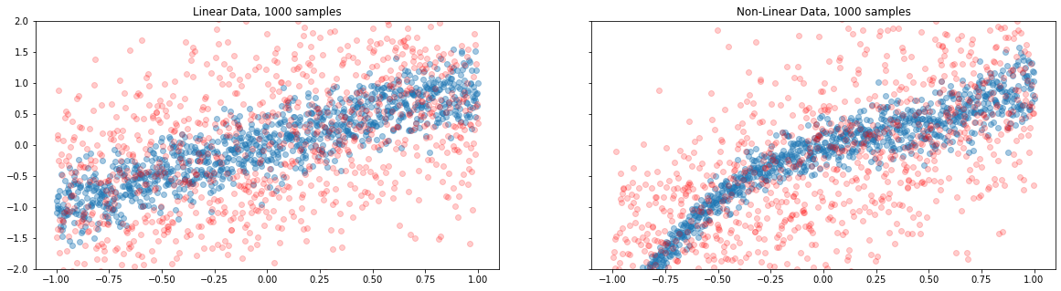
U.plot_deterministic_model_output(
    x_lin, y_lin, x_non_lin, y_non_lin, 
    n_samples, det_lin_reg_model, det_non_lin_reg_model
)

Here we go, a point function estimate identifies a line that minimize the error but missed the trend.

In deterministics models, deep neural networks converge based on a single value(of weights) to arrive at local minima. This is a major drawback due to which we often face poor model performance.

On fitting the linear and non linear datasets independently on the deteministic model, we have predicted the target values. The fitted line in red clearly shows the residuals. Though the model outputs are reasonable fine with the linear data, trend is not captured well with the non linear data. Needless to remind, almost all systems are non linear in nature.

This behaviour encourages one to arrive at finer algorithms to reduce the uncertainty.

Probabilistic Model

In deterministic models, each weight has a fixed(single) value to perform the backpropagation algorithm. On contrary, each weight is assigned with a distribution in a Probabilistic Model as shown in this figure.

Image Credit: Weight Uncertainty in Neural Networks

The distribution of a model parameter can be calculated using Bayesian Inference for the given data as follows

$$ P(w | D) = \frac{P(D | w) P(w)}{P(D)}. $$

where,

• $w$ is the model weights
• $D$ is the evidence, ie the given data. In our simulated synthetic data D is $D = {(x_1, y_1), \ldots, (x_n, y_n)}$
• $P(w)$ is the prior probability. That is the probability estimated prior observing the data
• $P(D|w)$ is the likelihood. The probability of observing the data $D$ for a given weight $w$. ie How good the model is
• $P(w|D)$ is the posterior probability. It is the distribution of model weight for a given data $D$

Bayes’ theorem gives us a way of combining data with some “prior belief” on model parameters to obtain a distribution for these model parameters that considers the data, called the posterior distribution. - Kevin Webter and team

Conditional Probability, explained…

Image Credit: xkcd

Probabilistic Linear Regression

Let us build a Probabilistic NN with one dense layer and a distribution lambda layer. The distribution layer in this model sets the mean from the data and constant variance to it.

negloglik = lambda y, rv_y: -rv_y.log_prob(y)

def probabilitic_lin_reg_model():
    model = tf.keras.models.Sequential([
        tf.keras.layers.Dense(units=1, input_shape=(1,)),
        tfpl.DistributionLambda(
            lambda t: tfd.Independent(tfd.Normal(loc=t, scale=1))
        )
    ])
    model.compile(
        loss=negloglik, 
        optimizer=tf.keras.optimizers.RMSprop(learning_rate=0.005)
    )
    return model

prob_lin_reg_model = probabilitic_lin_reg_model()
prob_lin_reg_model.fit(x_lin, y_lin, epochs=200, verbose=False)

prob_non_lin_reg_model = probabilitic_lin_reg_model()
prob_non_lin_reg_model.fit(x_non_lin, y_non_lin, epochs=200, verbose=False)

U.plot_probabilistic_model_output(
    x_lin, y_lin, x_non_lin, y_non_lin, 
    n_samples, prob_lin_reg_model, prob_non_lin_reg_model
)

The above plot clearly demonstrates the distribution of outcomes and how far they are from the observed target variables. This is a big revelation, and the reason for poor model performances. To be precise, though we learnt the mean reasonably well… spread out of the outcomes are haphazard. This behaviour indicates, the goal of learning is just not the mean but the spread out and beyond.

We shall further improve the model by fixing the variance in the final layer

def probabilitic_lin_reg_fixed_variance():
    model = tf.keras.models.Sequential([
        tf.keras.layers.Dense(input_shape=(1,), units=8, activation='sigmoid'),
        tf.keras.layers.Dense(tfpl.IndependentNormal.params_size(event_shape=1)),
        tfpl.IndependentNormal(event_shape=1)
    ])
    model.compile(
        loss=negloglik, 
        optimizer=tf.keras.optimizers.RMSprop(learning_rate=0.01)
    )
    return model

prob_lin_reg_fxvar_model = probabilitic_lin_reg_fixed_variance()
prob_lin_reg_fxvar_model.fit(x_lin, y_lin, epochs=500, verbose=False)

prob_non_lin_reg_fxvar_model = probabilitic_lin_reg_fixed_variance()
prob_non_lin_reg_fxvar_model.fit(x_non_lin, y_non_lin, epochs=500, verbose=False)

U.plot_probabilistic_fxvar_model(
    x_lin, y_lin, x_non_lin, y_non_lin, 
    n_samples, prob_lin_reg_fxvar_model, prob_non_lin_reg_fxvar_model
)

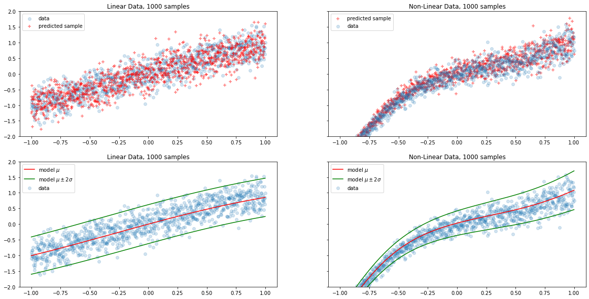
The above plots demonstrates the improvement in model due to the fact that it learned both the mean and the variance. .

With deterministic regression we obtained point estimates at the mean to predict the outcomes but we never had an idea about the aleatoric uncertainty. With probabilistic models we are able to evolve from point estimation at mean to a predicted distribution of the outcomes to minimized the uncertainty.

Epistemic Uncertainty

We have predicted a certain mean and a certain standard deviation for the above linear and non-linear synthetic data. In the space, there are many lines(predicted outcomes) could possibly generate the specific synthetic data of interest. The uncertainty caused due to the presense of multiple lines is nothing but epistemic uncertainty.

In this section, we are using varational prior and variatonal posterior to demonstrate epistemic uncertainty

Since the prior is the weight distribution before observing data, we shall have $\mu=0$ and $\sigma=1$

def prior(kernel_size, bias_size, dtype=None):
    n = kernel_size + bias_size
    prior_model = tf.keras.models.Sequential([
        tfpl.DistributionLambda(
            lambda t: tfd.MultivariateNormalDiag(loc=tf.zeros(n), scale_diag=tf.ones(n))
        )
    ])
    
    return prior_model

Variational posterior built with trainable distribution. It is the weights the model is adhered to and we want to learn the distribution. This multivariate gaussian has full covarinace matrix.

def posterior(kernel_size, bias_size, dtype=None):
    n = kernel_size + bias_size
    posterior_model = tf.keras.models.Sequential([
        tfpl.VariableLayer(tfpl.MultivariateNormalTriL.params_size(n), dtype=dtype),
        tfpl.MultivariateNormalTriL(n)
    ])
    return posterior_model

What are we doing here?
In a DNN setting, It is not possible to use Bayes Method to calculate the true posterior. Hence we define a variational posterior which is an approximation to the true posterior. This approximation is further tuned to get closer to the true posterior.

def probabilitic_lin_reg_weight_uncertainty(x_train, prior, posterior):

    model = tf.keras.models.Sequential([
        tfpl.DenseVariational(units=8,
                              input_shape=(1,),
                              make_prior_fn=prior,
                              make_posterior_fn=posterior,
                              kl_weight=1/x_train.shape[0],
                              activation='sigmoid'),
        tfpl.DenseVariational(units=tfpl.IndependentNormal.params_size(1), # Epistemic
                              make_prior_fn=prior,
                              make_posterior_fn=posterior,
                              kl_weight=1/x_train.shape[0]),
        tfpl.IndependentNormal(1) # Aleotoric
    ])
    model.compile(
        loss=negloglik, 
        optimizer=tf.keras.optimizers.RMSprop(learning_rate=0.005)
    )
    return model

x_lin_100, y_lin_100, x_non_lin_100, y_non_lin_100 = U.create_synthetic(n_samples=100, show_plots=False)
x_lin_1000, y_lin_1000, x_non_lin_1000, y_non_lin_1000 = U.create_synthetic(n_samples=1000, show_plots=False)

lin_model_100 = probabilitic_lin_reg_weight_uncertainty(x_lin_100, prior, posterior)
lin_model_100.fit(x_lin_100, y_lin_100, epochs=1000, verbose=False)

non_lin_model_100 = probabilitic_lin_reg_weight_uncertainty(x_non_lin_100, prior, posterior)
non_lin_model_100.fit(x_non_lin_100, y_non_lin_100, epochs=1000, verbose=False)

lin_model_1000 = probabilitic_lin_reg_weight_uncertainty(x_lin_1000, prior, posterior)
lin_model_1000.fit(x_lin_1000, y_lin_1000, epochs=1000, verbose=False)

non_lin_model_1000 = probabilitic_lin_reg_weight_uncertainty(x_non_lin_1000, prior, posterior)
non_lin_model_1000.fit(x_non_lin_1000, y_non_lin_1000, epochs=1000, verbose=False)

<tensorflow.python.keras.callbacks.History at 0x7fd5e8ba48e0>

U.plot_epistemic_uncertainty(
    x_lin_100, y_lin_100, x_lin_1000, y_lin_1000, 
    x_non_lin_100, y_non_lin_100, x_non_lin_1000, y_non_lin_1000,
    lin_model_100, lin_model_1000, 
    non_lin_model_100, non_lin_model_1000
)

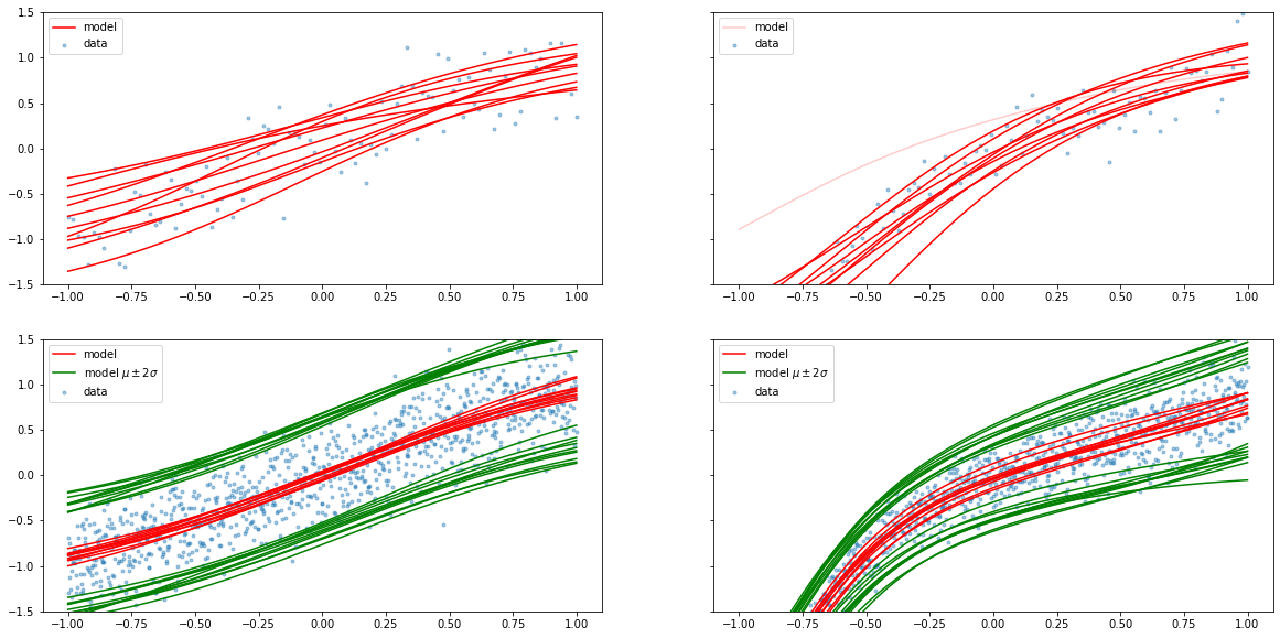
Above plot infers, with more data - Epistemic uncertainty can be minimized.

Inference

In this post,

1. Built 4 models to demonstrate deterministic and probabilistic regression on linear and non linear data
2. Witnessed the limitations of point functions over weight distributions during learning
3. Proved uncertainty by visually demonstrating multiple possible inputs for a single outcome
4. Constructed neural networks with prior and posterior probabilities

Reference

• Probabilistic Deep Learning with TensorFlow 2, I recommend this course if you are interested in quick start probilistic deep learning
• Weight Uncertainty in Neural Networks