In this post - we shall summarize some of the biological inspirations that led to break through in building intelligent systems, especially The Spiking Neuron. This post is part of the neuroscience series where we earlier explored post-synaptic depression mechanism of synaptic plasticity.

• Understanding Post-Synaptic Depression through Tsodyks-Markram Model by Solving Ordinary Differential Equation

Trivia

Neocortex
Neocortex is the boss of all bosses in the human nervous system. It performs higher functions like sensory perception, generation of motor commands, spatial reasoning, conscious thought, language processing etc.
Thalamas
Thalamas in the human brain is known for process and relay sensory informations like visual, auditory, somatosensory systems. It also plays a significant role in motor activity, emotion, memory, arousal and other associated functions.
Mammalian Brain, Rat
Spiking neuron model is built based on the firing patterns observed and recorded from the rat’s motor cortex.

Image Credit: Neural Networks 4: McCulloch & Pitts neuron - Victor Lavrenko

Objective

• Overview of various bilogically inspired intelligent systems
• Geometrical interpretation of McColloch-Pitt’s model
• Biophysics through Hodgkin-Huxley Model
• Rosenblatt’s perceptron, the inspiration for DNN
• What is Hebbian theory?
• Nature of a Spiking Neuron
• Build and simulate spiking neurons

Introduction

Our goal is to model a simple spiking neuron, which is biologically plausible, computationally efficient that integrates to form a cluster of neurons. This spiking neuron model is built by taking inspiration from various models that are demonstrated during the last few decades. We shall see an overview of the following models/theory that is foundational to computational neuroscience.

• McColloch-Pitts Model
• Hodgkin-Huxley Model
• Rosenblatt’s Model
• Hebbian Theory

McColloch-Pitts Model

McColloch-Pitts model is the first neuronal model proposed by Warren McCulloch a neuro-scientist and Walter Pitts a logician in 1943. It takes the input from synapses and dendrites having two parts ${g,f}$. Inputs are fed to $g$ and aggregated, based on the value of aggregated result $f$ makes a decision.

Image Credit: McCulloch-Pitts Neuron — Mankind’s First Mathematical Model Of A Biological Neuron

$$g(x_1, x_2, x_3, \cdots, x_n) = g(x) = \sum_{i=1}^n x_i$$ $$i.e.$$ $$y = f(g(x)) = \begin{cases} 1 & \text{if } g(x) \geq \theta, \ 0 & \text{if } g(x) < \theta \end{cases} \tag{1. McColloch-Pitts Model}$$

Where $\theta$ is nothing but some threshold.

Geometrical Interpretation of MP Model

A single McCulloch Pitts Neuron can be used to represent boolean function which are linearly separable. i.e. there exists a line(or plane) such that all inputs in which produce a 1 lie on one side of the line(plane) and all inputs which produce a 0 lie on other side of the line (plane).

Image Credit: McCulloch-Pitts Neuron — Mankind’s First Mathematical Model Of A Biological Neuron

As mentioned earlier, MP models are designed to solve boolean functions. For e.g. Whether it will rain or not? Whether AI will takeover the world or not? etc. Linear separation for a 3D space is a 2D plane, geometrically demonstrated here.

Image Credit: McCulloch-Pitts Neuron — Mankind’s First Mathematical Model Of A Biological Neuron

MP models has the following limitations,

• non boolean functions like regression functions,
• when all inputs are equal and
• if the functions are not linearly separable(XOR).

Hodgkin-Huxley Model

In 1952, Hodgkin and Huxley demonstrated a mathematical model comprises of non-linear differential equations that approximates the electrical characteristics of an excitatory neurons at intra/extracellular level. This model is a continous time dynamical system. Following are the components of the model

Image Credit: Hodgkin–Huxley model - Wikipedia

$$I_c = C_m \frac {dV_m}{dt}$$

• $I_c$ is the current flowing through the lipid bilayer
• $C_m$ is capacitance of the lipid bilayer
• $V_m$ is the membrane potential

$$I_i = g_i(V_m - V_i)$$

• $I_i$ is the current through an ion channel
• $g_i$ is the conductance of the ion channel and
• $V_i$ is the reverse potential of the i-th ion channel

The total current through the membrane is a function of potassium and sodium reversal potentials. $$I = C_m \frac {dV_m}{dt} + g_K(V_m - V_K) + g_{Na}(V_m - V_{Na}) + g_l(V_m - V_l) \tag{2.Hodgkin Huxley Model}$$

Where

• $g_{K, Na, l}$ are Potassium, Sodium and Leak channel conductances respectively
• $V_{K, Na, l}$ are Potassium, Sodium and Leak channel potentials respectively

Hodgkin-Huxley model demonstrates the neuronal behaviour precisely, making it a biologically plausible one. However spiking and bursting behavior of cortical neurons are modeled by Eugene M. Izhikevich by having Hodgkin-Huxley model as the basis. This model can simulate tens of 1000s of spiking neurons in realtime.

Rosenblatt’s Model

In 1958, Frank Rosenblatt demonstrated the first artificial neuron using a punch card system that learns through iteratively updating the weights. It took 50 trials to converge and we celebrate this model as the first single layer perceptron. In modern day interpretation, it is a binary classifier based on a threshold function,

Image Credit: Rosenblatts-perceptron

$$f(x) = \begin{cases} 1 & \text{if } w.x + b > 0, \ 0 & otherwise \end{cases} \tag{3. Rosenblatt’s Model}$$ Where,

• $w$ is a vector of real-valued weights
• $w.x$ is the dot product $\sum_{i=1}^m w_ix_i$, m is the number of inputs to the perceptron
• $b$ is the bias that shifts the decision boundary away from the origin and independent of the input

Rosenblatt’s model is considered to be the foundation for modern day deep learning systems through backpropagation algorithm.

Hebbian Theory

Hebbian theory states “Neurons that fire together wire together”, it claims an increase in synaptic efficacy arises from a presynaptic cell’s repeated stimulation of postsynaptic cell. It is the adaptation of neurons during the learning process through synaptic plasicity. Hebb states it as follows,

Let us assume that the persistence or repetition of a reverberatory activity (or "trace")
tends to induce lasting cellular changes that add to its stability. ... When an axon of cell
A is near enough to excite a cell B and repeatedly or persistently takes part in firing it, 
some growth process or metabolic change takes place in one or both cells such that A's 
efficiency, as one of the cells firing B, is increased
- Donald Hebb in his 1949 book, The Organization of Behavior

From an ANN point of view, it is a method to determine the weights between the neurons. i.e. Weight between two neurons increases if those 2 neurons activate simultaneously and reduces if they activate separately. $$w_{ij} = x_ix_j \tag{4. Hebbian Weight}$$ where,

• $w_{ij}$ is the weight of the connection from $neuron_j \rightarrow neuron_i$
• $x_i, x_j$ are the inputs to the neurons $i,j$

Let us say, there are $p$ training patterns and then the equation evolves to $$w_{ij} = \frac {1}{p} \sum_{k=1}^p x_i^kx_j^k$$

Spiking Neuron

In this section, we shall understand the function of a spiking neuron. Based on Hodgkin-Huxley model and Hebbian Theory, we shall simulate various types of spiking neurons based on Eugene Izhikevich’s 2003 IEEE paper titled Simple Model of Spiking Neurons.

When the membrane potential reaches the threshold, the neuron fires, and generates 
a signal that travels to other neurons which, in turn, increase or decrease their 
potentials in response to this signal. A neuron model that fires at the moment of 
threshold crossing is also called a spiking neuron model.
- Wikipedia

Image Credit: Dynamical Systems in Neuroscience by Eugene M. Izhikevich

A neuron received inputs from more than 10,000 other neurons through the contacts on its 
dendritic tree called synapses. The inputs produce electrical transmembrane currents that 
change the membrane potential of the neuron. Synaptic current produce changes, called post 
synaptic potentials (PSPs). Small currents produce smapp PSPs, larger currents produce 
significant PSPs that can be amplified by the voltage sensitive channels embedded in the 
neuronal membrane and lead to the generation of an action potential or spike - an abrupt 
and transient change of membrane voltage that propagates to other neurons via a long 
protrusion called an axon. Such spikes are the  main means of communication between neurons.

-Dynamical Systems in Neuroscience by Eugene M. Izhikevich

Simple Model of Spiking Neurons

In 2003 Izhikevich demonstrated a model that reproduce firing pattern of neurons recored from the rat’s motor cortex. Izhikevich says we need to combine experimental studies of animal annd human nervous systems with numerical simulation of large-scale brain models. The high level object of this model is to ensure

• Computationally Simplicity
• Capable of producing rich firing patterns exhibited by real biological neurons

By in large, Hodgkin-Huxley model is biophysically accurate but computationally prohibitive due to the restriction in number of neurons that can be simulated in real time. There are 2 key electrophysiological concepts that are foundational to the spiking neurons model,

• Bifurcation Parameter: When the amplitude is small, the cell is quiescent; when the amplitude is large, the cell fires repetitive spikes and
• Integrate and Fire: As the name suggests, together the neuronal cluster fires.
  The nuances of above topics are beyond the scope of this article, a deeper explanation of them are presented by Izhikevich in his book Dynamical Systems in Neuroscience.

The Model

Bifurcation methodologies plays significant role in simplifying Hodgkin-Huxley model to a 2-dimensional system of ordinary differential equations of the form

$$\large v’ = 0.04v^2 + 5v + 140 - u + I \tag{5}$$ $$\large u’ = a(bv - u) \tag{6}$$ with the auxiliary after-spike resetting $$\large \text{if } v \geq 30 mV, then \begin{cases} v \leftarrow c \ u \leftarrow u + d \end{cases} \tag{7}$$

where,
Dimensionless Variables

• $v$ represents the membrane potential of the neuron
• $u$ represents a membrane recovery variable,
• $I$ Synaptic DC current injected due to difference in potential

Dimensionless Parameters

• $a$ describes the time scale of the recovery variable $u$
• $b$ describes the sensitivity of the recovery variable $u$ to the fluctuations of the membrane potential $v$
• $c$ describes the after spike rest value of $v$ caused by high threshold $K^+$ conductance
• $d$ describes after-spike reset of the recovery variable $u$ caused by slow high-threshold $Na^+$ and $K^+$ conductances

The choices of these parameters determines various spiking patterns.

When the spike reaches the 30mV apex, the membrane voltage and the recovery variable are reset Ref: $eq.3$

Image Credit: Simple model of spiking neurons

Significance of the Variables ${u, v}$ and Parameters ${a, b, c, d}$

• $u$ accounts for the activation of $K^+$ ionic currents and inactivation of $Na^+$ ionic currents
• $u$ provides negative feedback to $v$
• Resting potential of the model is between $-70mV$ and $-60mV$
• Time is measured in $ms$ sale
• Threshold potential is not fixed, it ranges from $-55mV$ to $-40mV$
• $b$: Greater value of it couple $v$ and $u$ strongly and causes oscillations

$$\text{optimum values for the parameters}$$ $$\Large {a=0.02, b=0.2, c=-65mV, d=2}$$

With these details in hand, let us build the spiking neurons model.

Model Construction

Let us write 3 methods that satisfies the following logics, $$v’ = 0.04v^2 + 5v + 140 - u + I \tag{5}$$ $$u’ = a(bv - u) \tag{6}$$ $$\text{if } v \geq 30 mV, then \begin{cases} v \leftarrow c \ u \leftarrow u + d \end{cases} \tag{7}$$

# 𝑣′= 0.04𝑣^2 + 5𝑣 + 140 − 𝑢 + 𝐼
def calc_membrane_potential_v(prev_membrane_potential, membrane_recovery, synaptic_current):
    return 0.04 * (prev_membrane_potential ** 2) + 5 * prev_membrane_potential + 140 - membrane_recovery + synaptic_current

# 𝑢′=𝑎(𝑏𝑣−𝑢)
def calc_membrane_recovery_u(time_scale_recovery_a, sensitivity_uv, membrane_potential, membrane_recovery_prev):
    return time_scale_recovery_a * (sensitivity_uv * membrane_potential - membrane_recovery_prev)

# if 𝑣≥30𝑚𝑉, then 𝑣←𝑐, 𝑢←𝑢+𝑑
def calc_after_spike_reset(v, u, c, d):
    if(v > 30):
        v = c;
        u = u + d    
    return u, v

Ordinary Differential Equation - Step Function

Single step of length TIME_DELTA is multiplied to solve the differential equation.

def step_fn(u, v, a, b, c, d, t, I):
    u = u + t * calc_membrane_recovery_u(a, b, v, u)
    v = v + t * calc_membrane_potential_v (v, u, I)
    u, v = calc_after_spike_reset(v, u, c, d)
    
    return u, v

Simulation

ODE Simulate

Iterate through the steps and calculate ${u_t, v_t, I_t}$

def run(a, b, c, d, I, STEPS, TIME_DELTA):
    u = 0;
    v = 0;
    _v_t = []
    _u_t = []
    _I_t = []
    
    for j in range(0, STEPS):
        current = I[0]
        if (len (I) > 1):
            I = I[1:]
        u, v = step_fn(u, v, a, b, c, d, t=TIME_DELTA, I=current)
        _v_t.append(v)
        _u_t.append(u)
        _I_t.append(current)
        
    return _v_t, _u_t, _I_t

import matplotlib.pyplot as plt

def plot (_v_t, _u_t, _I_t, title, axs):
    axs.plot(_v_t, linestyle='solid')
    axs.plot(_u_t, linestyle='dashdot')
    axs.plot(_I_t, linestyle='dashdot')
    axs.legend(['$v_t$', '$u_t$', '$I_t$'], loc='lower right')
    axs.set_xlabel('ms')
    axs.set_ylabel('mV')
    axs.set_title(title)

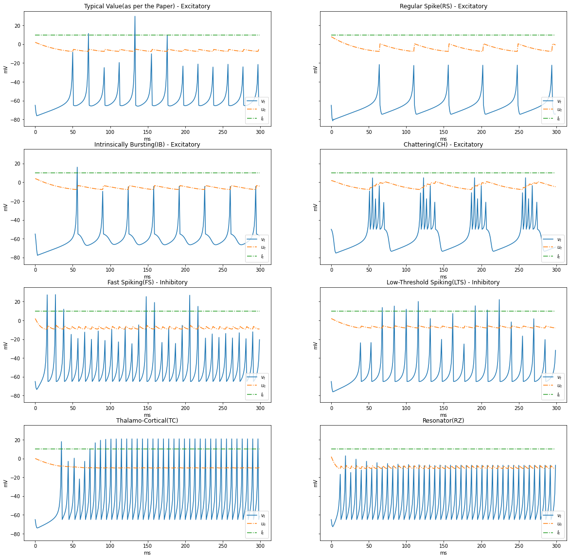
Types of Dynamics

Based on the patterns of spiking, neocortical neurons are classified. These are observed and recorded at intercellular level during spiking and bursting. The major classifcation of neurons in mammalian brain is 2, they and their subclasses as follows

• Excitatory Cortical Cells and
  • Regular Spiking(RS), most typical neurons in the cortex
  • Intrinsically Bursting(IB), stereotypical burst of spikes followed by repetitive single spikes
  • Chattering(CH), stereotypical bursts of closedly spaced spikes
• Inhibitory Cortical Cells
  • Fast Spiking(FS), fire periodic trains of action potentials with extremely high frequency without any slowing down
  • Low-Threshold Spiking(LTS), fire high frequency trains of action potentials, with a noticeable spike frequency adaptation.

Further our model reproduces the behaviour Thalamo-Cortical Neurons(TC) with two firing regimes(1 is demonstrated below) and Resonator Neurons(RZ).

Below graphs demostrates the behaviour of the various types of neurons.

neuron_types = {
    "Typical Value(as per the Paper) - Excitatory": {
        "a": 0.02, "b": 0.2, "c": -65, "d": 2
    },
    "Regular Spike(RS) - Excitatory": {
        "a": 0.02, "b": 0.2, "c": -65, "d": 8
    },
    "Intrinsically Bursting(IB) - Excitatory": {
        "a": 0.02, "b": 0.2, "c": -55, "d": 4
    },
    "Chattering(CH) - Excitatory": {
        "a": 0.02, "b": 0.2, "c": -50, "d": 2
    },
    "Fast Spiking(FS) - Inhibitory": {
        "a": 0.1, "b": 0.2, "c": -65, "d": 2
    },
    "Low-Threshold Spiking(LTS) - Inhibitory": {
        "a": 0.02, "b": 0.25, "c": -65, "d": 2
    },
    "Thalamo-Cortical(TC)": {
        "a": 0.02, "b": 0.25, "c": -65, "d": 0.05
    },
    "Resonator(RZ)": {
        "a": 0.1, "b": 0.26, "c": -65, "d": 2
    }
}
def render_dynamics(time_delta, steps, I):
    fig, axs = plt.subplots(4, 2, figsize=(20, 20), sharey=True)
    row = 0
    col = 0
    for name, params in neuron_types.items():
        _v_t, _u_t, _I_t = run(a=params["a"], b=params["b"], c=params["c"], d=params["d"], I=I, STEPS=steps, TIME_DELTA=time_delta)
        plot(_v_t, _u_t, _I_t, name, axs[row, col])

        col += 1
        if(col == 2):
            row += 1
            col = 0
            
TIME_DELTA = 1 # 1ms
STEPS = 300
I = [10] * STEPS

render_dynamics(TIME_DELTA, STEPS, I)

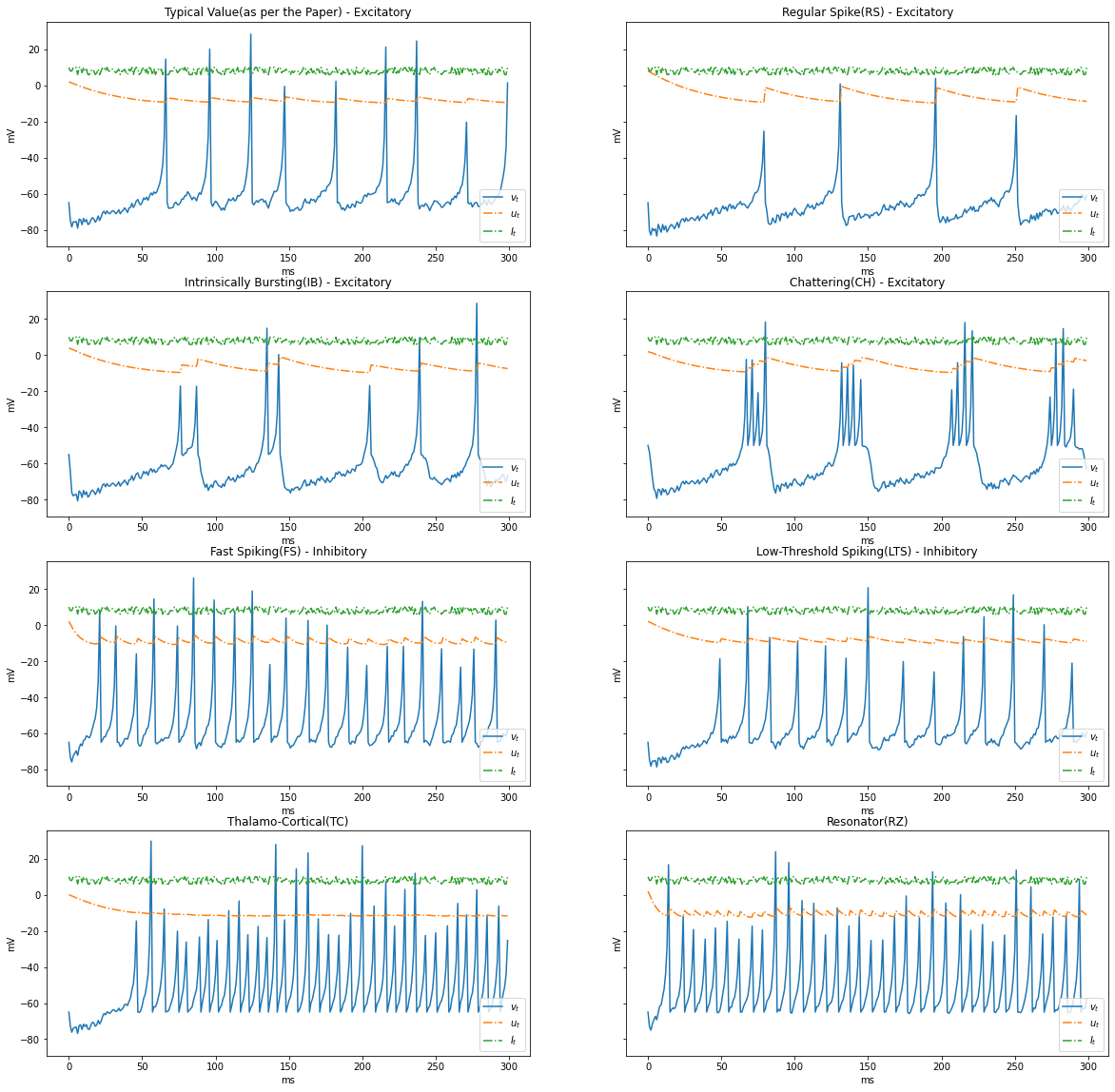
Varying $I_t$

In the previous simulation we had constant current, Let us experiment with a varying current between ${5, 10}$

import numpy as np
I = np.random.choice(np.arange(6, 11, 1), STEPS)
render_dynamics(TIME_DELTA, STEPS, I)

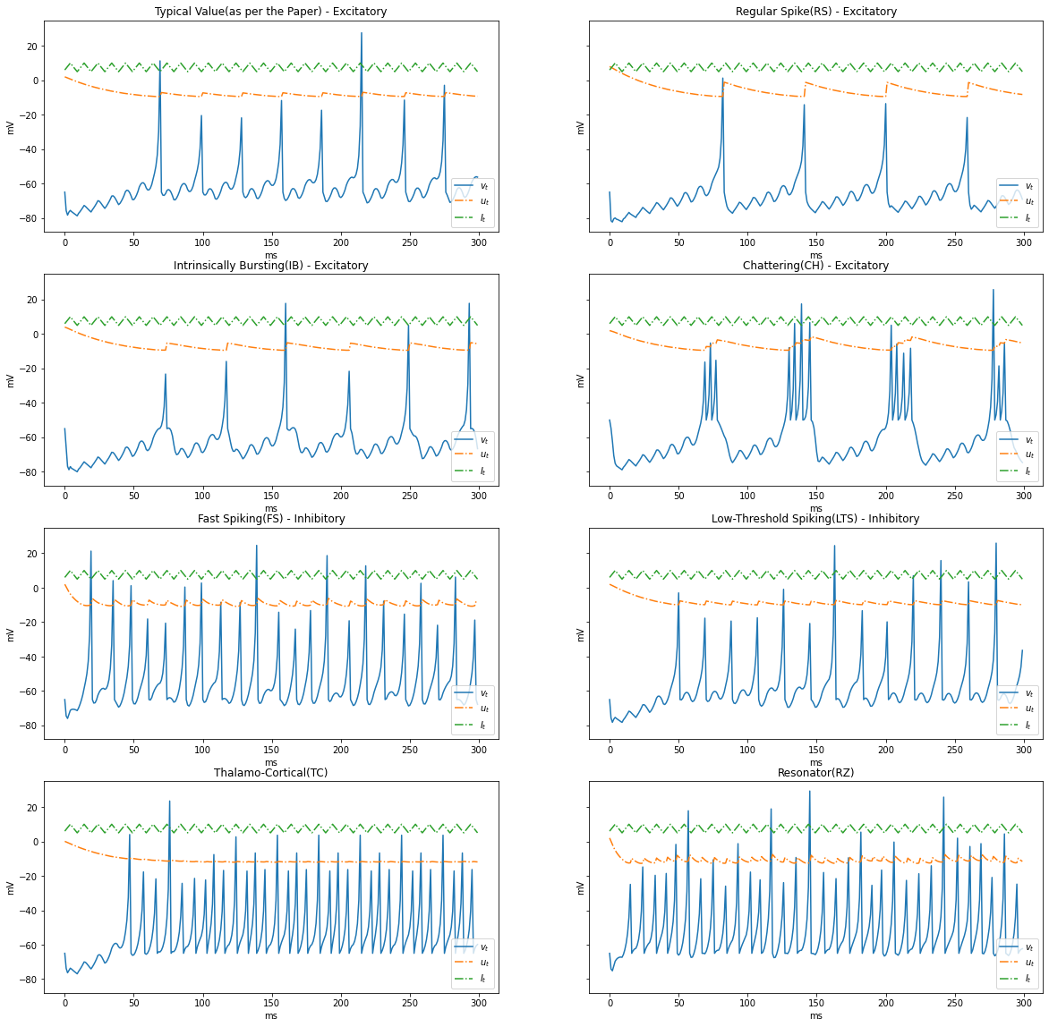
Surge and Sink $I_t$

Let us simulate a condition where current surges and sinks cyclically, $5 \rightarrow 10 \rightarrow 5$

I = np.tile(np.concatenate((np.arange(6, 11, 1),  np.arange(9, 4, -1))), STEPS//10)
render_dynamics(TIME_DELTA, STEPS, I)

Inference

In this post, we made an attempt to understand various biologically inspired neuronal models from as early as McColloch-Pitts’ Boolean Logic to Izhikevich’s Spiking Neurons. We also built the Spiking Neurons model and pondered over its simplicity and efficacy through various dynamics.
Future Work
I am planning to simulate the Pulse Coupled Implementation section in the paper where a cluster of 10,000 thalamo cortical neuronal network with 1M synaptic connections using a sparse network. Further, we can investigate the efficacy of Spiking Neural Networks and Neuromorphic Computing to understand the state of the art methodologies drawn from bilogical inspiration.

Reference

• Simple model of spiking neurons by Izhikevich, 2003 - IEEE Transactions of Neural Networks
• Hebbian theory from Wikipedia
• Perceptron from Wikipedia
• Rosenblatt’s perceptron, the first modern neural network by Jean-Christophe B. Loiseau
• McCulloch-Pitts Neuron — Mankind’s First Mathematical Model Of A Biological Neuron by Akshay L Chandra
• Recurrent Spiking Neural Network Learning Based on a Competitive Maximization of Neuronal Activity by Nekhaev et al, 2018 in Frontiers in Neuroinformatics
• Dynamical Systems in Neuroscience by Izhikevich, 2007