Shannon's Entropy, Measure of Uncertainty When Elections are Around
Posted April 3, 2021 by Gowri Shankar ‐ 6 min read
What is the most pressing issue in everyone's life, It is our inability to predict how things will turn out. i.e. Uncertainties, How awesome(or depressing) it will be if we make precise predictions and perform accurate computation to measure uncertainties.
This April is an Election Month for some of us… On which day you are certainly going to get fooled
- 1st of April or
- On the Day of Election
Measure of uncertainty is a function of probability.
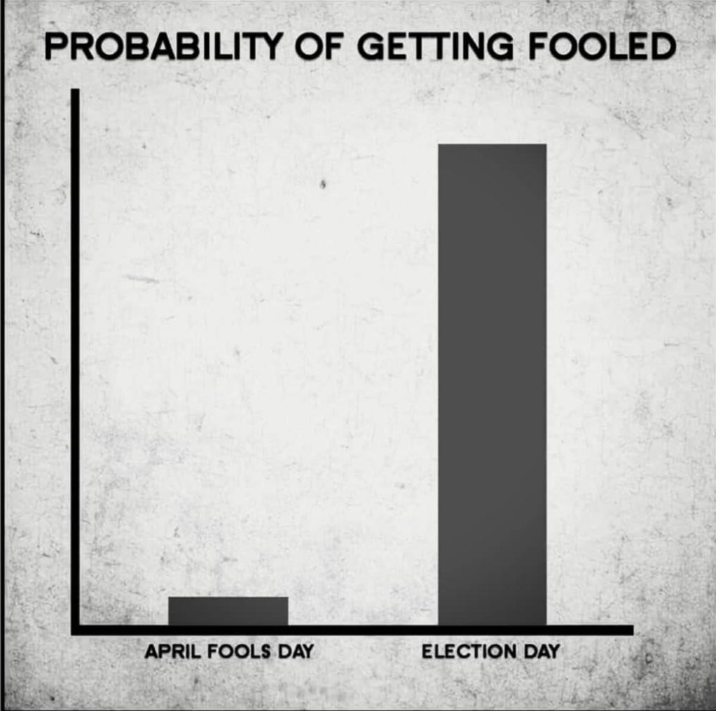 Image Credit: Dr.Raja
What’s your weekend plan? You have 2 days to chill, following are the given choices. How you will choose?
- Go on a hike to the nearby woods OR visit your nagging aunt in the nearby town
- Go on a hike to the nearby woods OR visit your loving parents in the nearby town
It looks, option 2 is the right choice at sight because it has more relevant choices within. However, it has the highest uncertainty compared to option 1. It is easy to pick what you want to do from the option 1 by deduction(empirically). In general, more relevant choices increases the uncertainty measure and our goal is minimizing uncertainty.
In this post let us understand entropy, measure of uncertainty to make right choices. Also introduce the concept of Gain used for reducing uncertainty.
This post is a continuation of my previous post on uncertainty titled
Understaning Uncertainty, Deterministic to Probabilistic Neural Networks and
Bayesian and Frequentist Approach to Machine Learning Models
Introduction
Claude Shannon came up with the theory of measuring uncertainty called entropy in his 1948 paper - We call it Shannon's Entropy($H$), It is also have one another name Expected Surprisal. Shannon’s Entropy defines axiomatic characterization of a discrete probability density function $P$ which gives event i probability $p_i$.
$$H(p_1, p_2, p_3, \cdots, p_N) \tag{1}$$ $$where$$ $$0 \leq p_i \leq 1$$ $$and$$ $$p_1 + p_2 + p_3 + \cdots + p_N = 1$$
- $eq.1$ is the measure of uncertainty($H$).
- N is the total number of events

Image Credit: Scientific American
Trivia: Shannon’s wife Betty a mathematician, Betty played significant role in Shannon’s success. She published her own research on “Composing Music by a Stochastic Process”. Eulogy for Betty in IEEE Information Theory Society Newsletter, P18
Shannon’s Theorem
Shannon proved the following fact…
Suppose $H(p_1, \cdots, p_N)$ is a function which satisfies the axioms discussed in the next section, Let $K=H(1/2, 1/2)$ when $N=2$, and define $0.log_2(0)=0$. Then $K \gt 0$, and for all N and all probability vectors $(p_1, \cdots, p_N)$
$$H(p_1, p_2, p_3, \cdots, p_N) = - \sum_{i=1}^n p_i log_2 p_i$$ Let us analyze few axioms that are insighful to understand Shannon’s.
import numpy as np
def entropy(p, is_total=True):
    epy = [p[i] * np.log2(p[i]) for i in np.arange(len(p)) if p[i] != 0]
    if(is_total == True):
        epy = -1 * np.sum(epy)
    return epy
entropy([0.3, 0.5, 0.2]), entropy([1/2, 1/2]), entropy([0.9, 0.1])
(1.4854752972273344, 1.0, 0.4689955935892812)
Axioms of Entropy
Uniform Distributions have Maximum Uncertainty
Let us say, probability($p_i$) of an event $i$ is $1/N$ for all N. i.e. Probability of going to nearby woods is equal to the probability of visiting your parents. Then it causes the maximum uncertainty $$A(N) = H(1/N, 1/N, \cdots, 1/N)$$
The above equation suggests, uniform distributions with more outcomes have more uncertainty. ie. $$H(Throwing Die) \gt H(Flipping Coin)$$ $$i.e.$$ $$H_N \left( \frac {1}{N}, \frac {1}{N}, \cdots, \frac {1}{N} \right) \lt H_{N+1} \left( \frac {1}{N+1}, \frac {1}{N+1}, \cdots, \frac {1}{N+1} \right) $$
Let us vaidate this axiom using our entropy function.
Case 1: Tossing a Fair Coin, Uniform Distribution
entropy([1/2, 1/2])
1.0
Case 2: Throwing a Fair Die, Uniform Distribution
entropy([1/6, 1/6, 1/6, 1/6, 1/6, 1/6]),
(2.584962500721156,)
Case 3: Some Random Uniform Distribution
randn = np.random.randint(1, 25, 1)
entropy(np.repeat(1/randn, randn)), randn
(4.584962500721156, array([24]))
Adding an Outcome with $0$ Probability has NO Effect
Let us say, there are 2 events and the probability$(p_2)$ of $2$nd event is zero. i.e. Visiting your nagging aunt is not a choice at all, then that probability has no effect. Complete certainty. $$H(p_1, p_2, p_3, \cdots, 0, \cdots, p_N) = H(p_1, p_2, p_3, \cdots, p_N)$$
entropy([0.3, 0.5, 0.2]), entropy([0.3, 0.5, 0.2, 0])
(1.4854752972273344, 1.4854752972273344)
Uncertainty is Additive for Independent Events
Let us say, Hiking to the nearby woods is an event and meeting your loving parents in the wood is another event. If hiking is independent of meeting your parents in the wood then the uncertainty of the events are sum of individual events $$H(Hiking2Woods, MeetingParents) = H(Hiking2Woods) + H(MeetingParents)$$
# Entropy of independent events are sum of their individual entropies
# i.e Entropy of tossing a coin and throwing a die
entropy([1/2, 1/2]) + entropy([1/6, 1/6, 1/6, 1/6, 1/6, 1/6])
3.584962500721156
Uncertainty Measure in Non-Negative
Uncertainty measures are non-negative. Lesser the entropy lesser the uncertainty. We shall proved this in the subsequent sections. $$H(X) = - \sum_{i=1}^n p_i log_2 p_i$$ Probabilities are positive and range between 0 and 1, log of probabilities are non-positive and we have a multiplication factor -1. Hence, entropy is non-negative for all inputs.
# Entropy for individual probabilites, log of probabilities are non positive
entropy([0.3, 0.5, 0.2], is_total=False)
[-0.5210896782498619, -0.5, -0.46438561897747244]
Lesser the Entropy, Lesser Uncertainty
Unfair Coin of probabilities 0.9 for Head and 0.1 for Tail compared with probabilities 0.6 for Head and 0.4 for Tail
entropy([0.9, 0.1]), entropy([0.6, 0.4])
(0.4689955935892812, 0.9709505944546686)
The measure of uncertainty is continuous in all its arguments
Measure of uncertainty is a continuous in the Cartesian plane, hence it is differentiable. Since it is continuous, changing the probability measure by a small fraction changes the entropy by a very small amount.
Until previous section, we spoke about discrete functions. Shannon replaced the summation symbol of discrete version into integral to make continuous
$$h(X) = - \int p(x)logp(x)dx$$
However Edwin Thompson Jaynes addressed various flaws of this function and derived by taking the limit of increasingly dense discrete distributions. Suppose we have set of $N$ discrete points, such that $N \rightarrow \infty$ their density approaches a function $m(x)$ called the invariant measure
$$H(X) = - \int p(x) log \frac {p(x)}{m(x)} dx$$
Conclusion
In this post we explored Entropy - The Measure of Uncertainty and the axioms of it. In Applied Machine Learning we focus on cross entropies.
Cross entropy is a famous loss function used in deep learning for classification and generation problems. It is generally refer to calculating the difference between two probability distributions. Cross Entropy is related to KL-Divergence and Log-Loss but not the same. We shall explore cross entropies in the future postsl.
I planned to cover the following topics as and when I get time - Let me know, If anything else to be covered.
- Entropy in ML: Decision Trees
- Entropy in ML: Calculating Gain, i.e. How to reduce uncertainty
- Entropy in Deep Learning: KL-Divergence

Image Credit: https://maxthedemon.com/